Formula to Return Blank Cell instead of Zero in Excel (with 5 Alternatives)
The easiest way to to return a blank cell instead of zero in Excel is to use a formula. In this article we’ll demonstrate and explain that formula, and provide 5 alternative methods.
Formula to Return Blank Cell instead of Zero: Combination of IF and VLOOKUP Functions
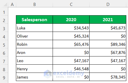
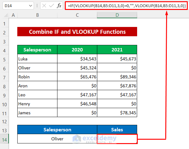
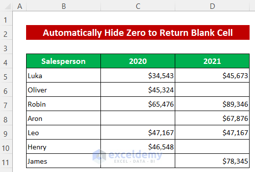
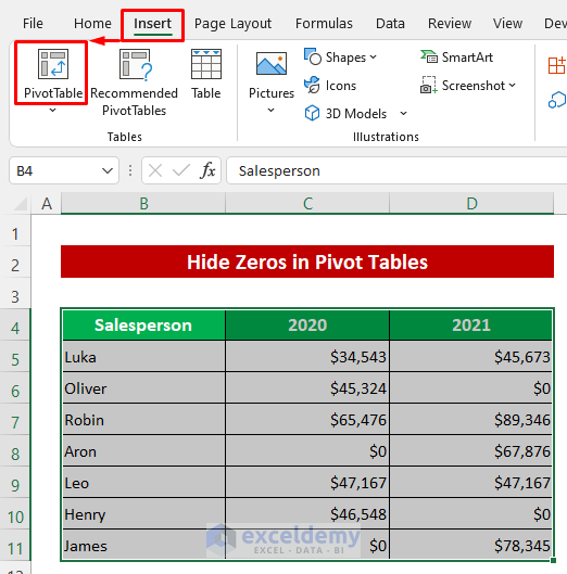
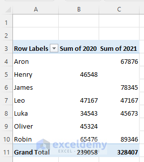
The following dataset contains some salespersons’ sales in two consecutive years. There are zero sales in some cells. We’ll use the IFand VLOOKUPfunctions in a formula to display blank cells in those cells instead. Steps:
- Enter the following formula in Cell D14:
=IF(VLOOKUP(B14,B5:D11,3,0)=0,"",VLOOKUP(B14,B5:D11,3,0))
The formula returns blank cells for the zero sales of Oliver.
Alternative Methods
Method 1 – Automatically Hide Zero
Excel has an built in feature that will convert all the zeros to blank cells automatically.
Steps:
 Cell in Excel" width="523" height="521" />
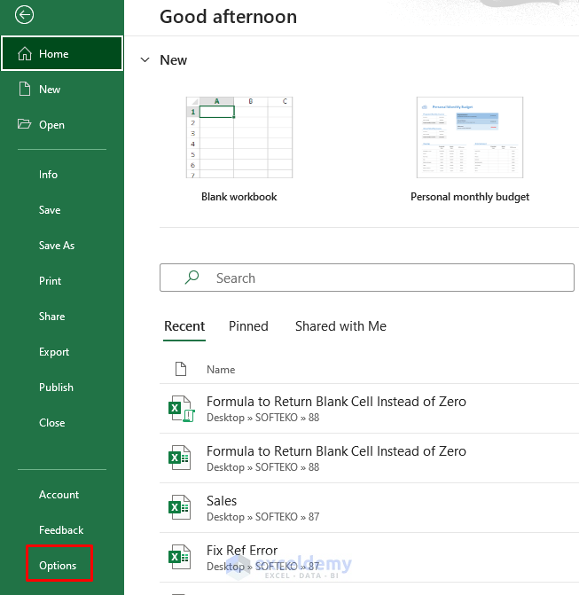
- Click Options from the bottom section, and a dialog box will open up.
 Cell in Excel" width="653" height="671" />
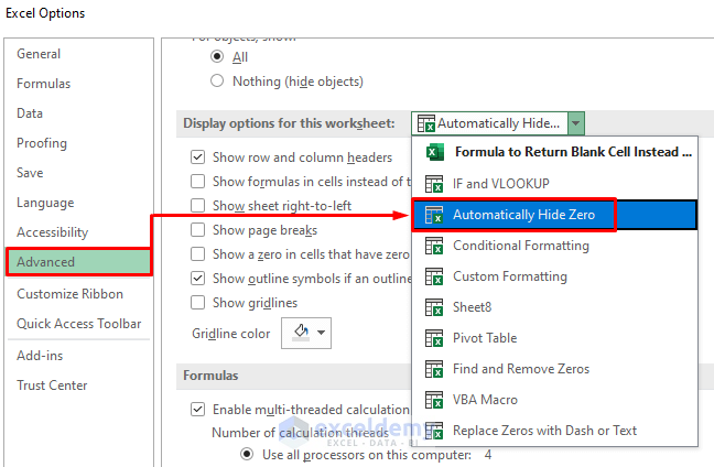
- Click the Advanced option.
- Select the sheet from the drop-down of Display options for this worksheet section.
 Cell in Excel" width="648" height="424" />
- Just unmark the Show a zero in cells that have zero value option.
- Click OK.
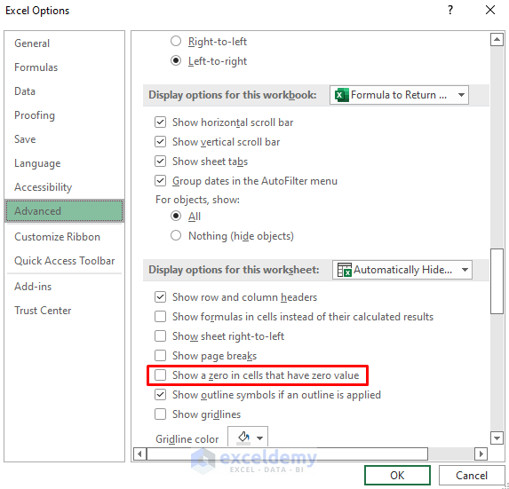
Blank cells will appear where all the zeros were before.
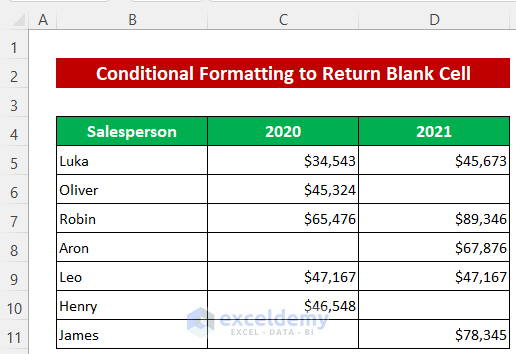
Method 2 – Using Conditional Formatting
Steps:
- Select the data range C5:D11.
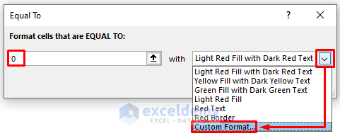
- Click as follows: Home > Conditional Formatting > Highlight Cells Rules > Equal To.
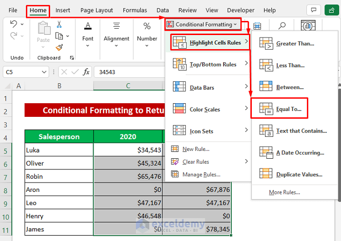
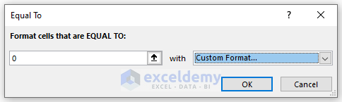
- Enter zero in the Format cells that are EQUAL TO box.
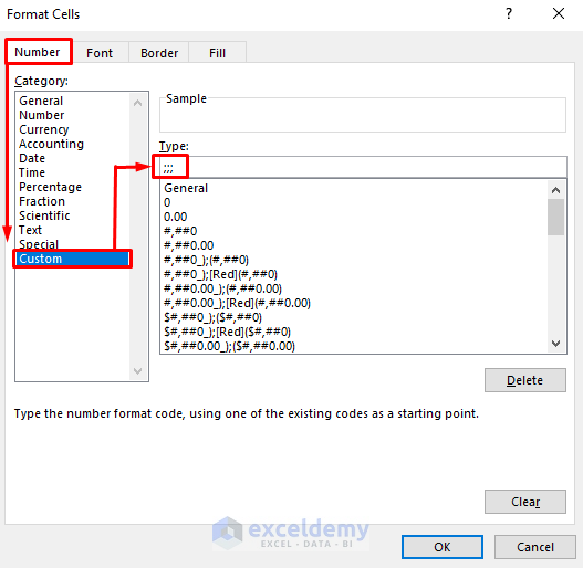
- Select Custom Format from the dropdown list.
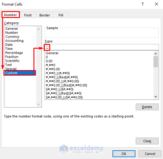
A Format Cells dialog box will open up.
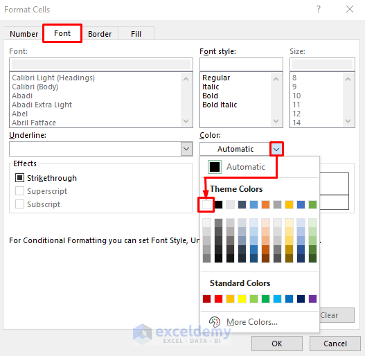
- Alternatively, click Number > Custom and type three semicolons (;;;) in the Type box.
- Click OK and it will return to the previous dialog box.
All the zero values are returned as blank cells.
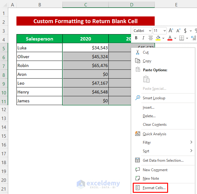
Method 3 – Apply Custom Formatting
Steps:
- Select the data range.
- Right-click your mouse and select Format Cells from the Context menu.
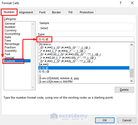
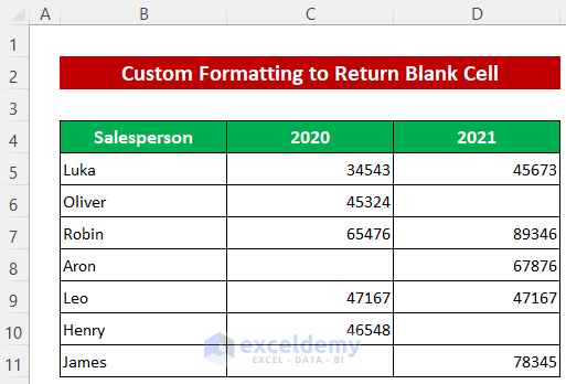
Blank cells now appear where the zeros were.
Method 4 – Using Pivot Tables
Steps:
- Select the whole dataset.
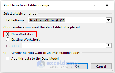
- Click Insert > Pivot Table.
- Select your desired worksheet and click OK (here, New Worksheet).
- Select the data range from the Pivot Table.
- Click as follows: Home > Conditional Formatting > Highlight Cells Rules > Equal To.
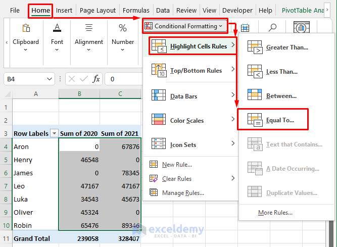
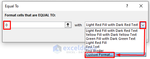
- Enter 0 (a zero) in the Format cells that are EQUAL TO box.
- Select Custom Format from the dropdown list.
A Format Cells dialog box will open up.
And we are done.
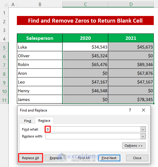
Method 5 – Using Find and Replace
Steps:
- Select the data range C5:D11.
- Press Ctrl+H to open the Find and Replace dialog box.
- Enter 0 (a zero) in the Find what box and keep the Replace with box empty.
 Find and Remove Zeros to Return Blank Cell in Excel" width="524" height="554" />
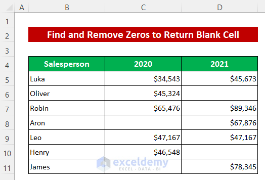
All the zeros are replaced with blank cells.
 Find and Remove Zeros to Return Blank Cell in Excel" width="524" height="356" />
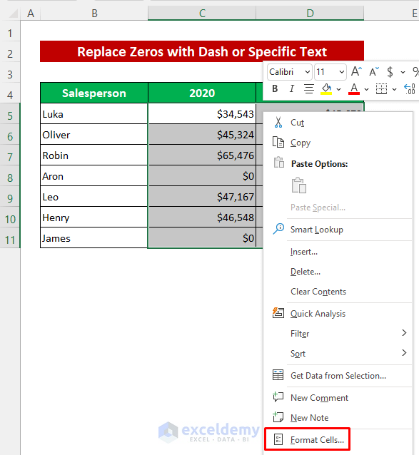
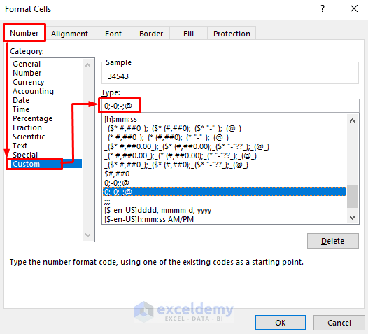
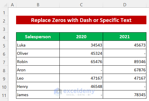
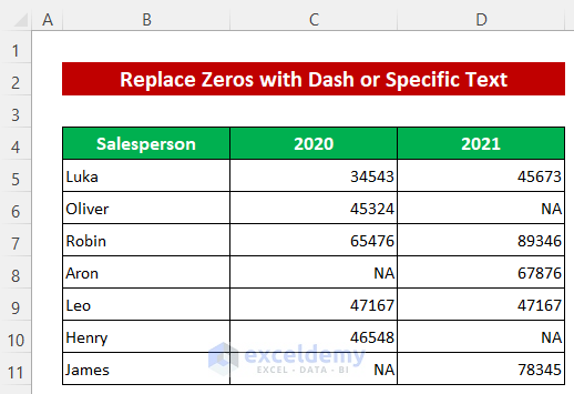
Replace Zeros with Dash or Specific Text
It’s as simple to replace zeros with a dash or specific text instead of blank cells.
Steps:
- Select the range of data.
- Right-click your mouse and select Format Cells from the Context menu.
The output will look like the image below.
- To return specific text, just replace the dash with whatever text you want within double quotes.
I typed NA.
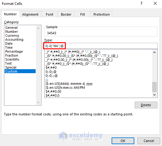
The zeros in the cells now display ‘NA’.
Download Practice Workbook
Formula to Return Blank Cell Instead of Zero.xlsx
Related Articles
- How to Find Blank Cells in Excel
- Null vs Blank in Excel
- How to Highlight Blank Cells in Excel
- How to Deal with Blank Cells That Are Not Really Blank in Excel
- Return Non Blank Cells from a Range in Excel
